Show the code
import numpy as np
from PIL import Image
from scipy.ndimage import convolve
from matplotlib.pyplot import imread
import matplotlib.pyplot as pltKashish Mukheja
Saturday, 27 May 2023
Pixel is the smallest fragment of an image.
Every pixel can store 8 bits of memory, for e.g. So, the range of values it can store is 2^8=256, i.e., between 0 to 255. Where 255 represents white shade, and 0 represents black shade. Numbers between 0 & 255 are different shades of black and white “OR” grey
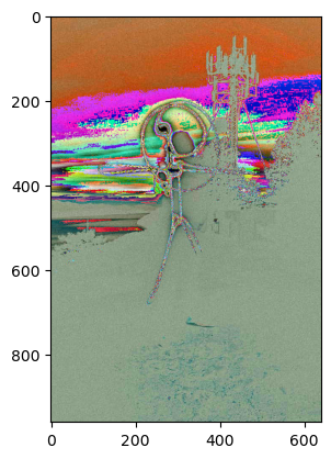
Filters are a way to alter the original image. Filters are smaller matrix that are multiplied with larger matrix in a left to right fashion (like a torch), for e.g., to result in a different matrix. The resultant matrix will have different pixel values at certain places which will result in altering the source image. This can be inferred as a small convolution operation. They are also termed as Kernels
These filters can help in detecting edges or differentiate between brightness.

# We have 3 channels since it's a colored image, hence we loop over 3 times.
# convolve(array_input, filter) will do the convolution operation, i.e.,
# multiply input image for each channel with the filter matrix
for channel in range(3):
    res = convolve(image_profile[:,:,channel], Edge)
    Image_channel.append(res)

img = np.dstack((Image_channel[0], Image_channel[1], Image_channel[2]))
plt.imshow(img)
plt.show()
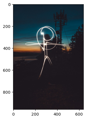
Shape of output image = (960, 640, 3)
Shape of input image = (960, 640, 3)
Length of Image channel = 3
Shape of each Image Channel = (960, 640)There are some in built filters present in PIL library :-
from PIL import Image, ImageFilter
from PIL.ImageFilter import (BLUR, CONTOUR, EDGE_ENHANCE...)There are mainly two reasons why convolution is required instead of having just a simple feed forward NN: 1. Humongous number of input parameters (i.e, pixel size) 2. Exploit the spacial correlation across pixels resulting in reducing in number of operations for NN.
A snapshot of input matrix (For E.g., 3 * 3) is convolved with a filter matrix (also 3 * 3), also called Weights. The actual input image can be of size say 10 * 10. The filter matrix will swipe through the entire input matrix taking a snapshot of 3 * 3 (just like how a torch moves from left to right and top to bottom). The resultant matrix is a colnvoluted matrix. “Colvolved” involes summation of dot product of two matrices. Convolution helps extracting characteristics in an image. It also helps to reduce computation because at every convolution operation, we are reducing the dimension of the image which will be eventually given as input to the neural network classifier.
Convolution combined with a feed forward network is called CNN. We applied convolution to N * M matrix.
Then we flatten the image to 1D( 1 * ( N * M ) ) and apply the normal feed forward neural network.
Adding additional rows/columns to the image arrays. This is usually done symmetrically. Zero-padding means adding Zeroes (i.e., black) pixels to the boundary of images.
This can be sometimes required when you don’t want to reduce the size of the output matrix once the filter is applied. For E.g., Input 100 * 100 matrix is multipled by 3 * 3 filter -> Resultant is 98 * 98 matrix. But if you want to keep the input image intact, you can add padding to the input image to make it 102 * 102.
This is also useful to provide all pixels equal importance, mainly the Edges of the image which are only multiplied with the filter twice, as compared to the inner regions which are multiplied three or more times.
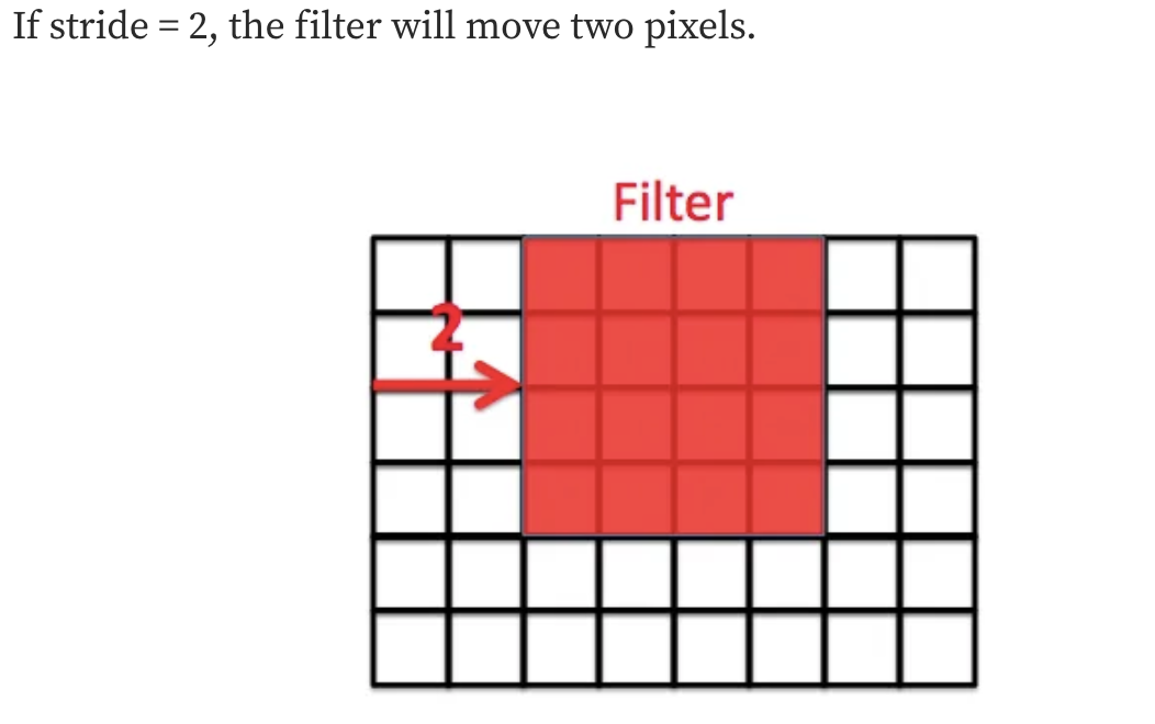
Stride is a parameter of the neural network’s filter that modifies the amount of movement over the image. Stride of 2 means the filter moves two pixels ahead, that is, 1 pixel is ignored. Stride of 1 is the default movement for filter, in which case no pixel is ignored.

Also type of sub-sampling, used to reduce the size of input image in multiplicative way. Max, Average and Min Pooling are two common type of pooling. In MaxPooling, the maximum value of the resultant 3 * 3 snapshot will be taken as the output pixel for that area.
Output of the convolution after doing all the operations like pooling, stride, padding, is called a feature map. This feature map is passed through an activation function like ReLU, and called an activation map.
Once the image has gone through N Convolution layers, it is flattened to feed into the fully connected neural network, which will then perform classification. Here, the learnable parameters weights are Filters. So, the filter weights are updated during backpropagation.