import matplotlib.pyplot as plt # We import matplotlib to generate bar plots
import numpy as npA Report by …
Name: Kashish MukhejaIntroduction
In this report, we conduct a comprehensive analysis of the BTC-USD exchange rates during the third quarter (Q3) of 2023. The analysis encompasses various aspects, including data extraction, statistical analysis, visualization, and outlier detection, with the aim of gaining insights into the price movements and trends observed during this period. The report addresses the following key concepts:
Loading and examining the dataset: We start by loading the dataset containing daily exchange rates from a CSV file and inspecting the data structure.
Statistical analysis: We calculate essential statistical metrics, such as mean, minimum, maximum, quartiles, standard deviation, and interquartile range, to characterize the distribution of exchange rates during Q3 2023.
Visualization of exchange rate trends: Using matplotlib, we create visualizations to illustrate the daily exchange rate trends throughout Q3 2023, facilitating a better understanding of price movements over time.
Identification of outliers: We employ box-and-whisker plots to detect outliers in the daily price changes and interpret their significance in the context of the exchange rate fluctuations observed during Q3 2023.
Data Preparation
To start with, let’s import the necessary libraries and load the bitcoin data from BTC-USD.csv file.
rates = np.loadtxt('BTC-USD.csv')
rates[:10]
array([16625.08008, 16688.4707 , 16679.85742, 16863.23828, 16836.73633,
16951.96875, 16955.07813, 17091.14453, 17196.55469, 17446.29297])We load the data using numpy’s loadtxt function and assign it to the variable rates.
Statistical Analysis of Q3 2023 Exchange Rates
This section extracts and analyzes exchange rate data for the third quarter of 2023, focusing on key statistical metrics such as mean, minimum, maximum, quartiles, standard deviation, and interquartile range.
# Extract data for rows 182 to 272 inclusive
selected_rates_q3 = rates[181:272+1]  # Python indexing is zero-based

# Calculate statistics
arithmetic_mean = np.mean(selected_rates_q3)
minimum = np.min(selected_rates_q3)
first_quartile = np.percentile(selected_rates_q3, 25)
median = np.median(selected_rates_q3)
third_quartile = np.percentile(selected_rates_q3, 75)
maximum = np.max(selected_rates_q3)
standard_deviation = np.std(selected_rates_q3)
interquartile_range = third_quartile - first_quartile

# Display the calculated statistics
print("Arithmetic Mean:", arithmetic_mean)
print("Minimum:", minimum)
print("First Quartile:", first_quartile)
print("Median:", median)
print("Third Quartile:", third_quartile)
print("Maximum:", maximum)
print("Standard Deviation (SD):", standard_deviation)
print("Interquartile Range (IQR):", interquartile_range)
Arithmetic Mean: 28091.328677608693
Minimum: 25162.6543
First Quartile: 26225.555665
Median: 28871.817385
Third Quartile: 29767.069825
Maximum: 31476.04883
Standard Deviation (SD): 1827.0403130479656
Interquartile Range (IQR): 3541.514159999999- We extract the desired rows using array slicing (rates_arr[181:272+1]) since Python indexing is zero-based.
- We calculate the required statistics using NumPy functions such as np.mean, np.min, np.percentile, np.median, and np.std.
Finally, we displayed the calculated statistics. As displayed above, the statistical summary included Arithmetic Mean, Min, Q1, Median, Q3, Maximum, Standard Deviation and Interquartile Range.
Visualization of Q3 2023 Exchange Rates
This section illustrates the trends in BTC-USD exchange rates from July 1st to September 30th, 2023, utilizing a line plot with red solid lines to represent the daily exchange rate fluctuations. > We assume index 182 represents July 1st and index 272 represents September 30th.
# Extract days and rates
days = np.arange(1, len(selected_rates_q3) + 1)  # Days from July 1st to September 30th
rates = selected_rates_q3

# Plot the data
plt.plot(days, rates, color='red', linestyle='-', label='Q3 2023')  # Red solid line
plt.title('BTC-USD Exchange Rates in Q3 2023')
plt.xlabel('Days (July 1st to September 30th)')
plt.ylabel('Exchange Rate')
plt.legend()
plt.show()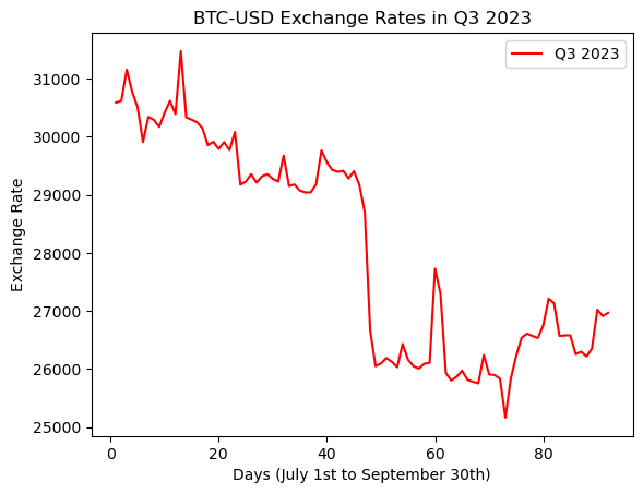
Identification of Lowest and Highest Observed Prices
We now determine the day numbers with the lowest and highest observed prices in Q3 2023, along with their corresponding price values, by finding the indices of the minimum and maximum values in the selected exchange rate data array.
# Find the index of the lowest observed price
lowest_price_index = np.argmin(selected_rates_q3)

# Find the index of the highest observed price
highest_price_index = np.argmax(selected_rates_q3)

# Calculate the corresponding day numbers (assuming index 182 denotes July 1st)
lowest_price_day = lowest_price_index + 182
highest_price_day = highest_price_index + 182

# Retrieve the lowest and highest observed prices
lowest_price = selected_rates_q3[lowest_price_index]
highest_price = selected_rates_q3[highest_price_index]

# Print the results
print("Lowest price was on day", lowest_price_day, "(", lowest_price, ").")
print("Highest price was on day", highest_price_day, "(", highest_price, ").")
Lowest price was on day 254 ( 25162.6543 ).
Highest price was on day 194 ( 31476.04883 ).Visualization of Q3 2023 Daily Price Changes
Let’s dive a bit further in this section. It presents a horizontal box-and-whisker plot illustrating the distribution of daily price increases and decreases during Q3 2023. The arithmetic mean of the price changes is marked on the plot with a green “x”.
import numpy as np
import matplotlib.pyplot as plt

# Compute daily price changes for Q3 2023
price_changes = np.diff(selected_rates_q3)

# Create a horizontal box-and-whisker plot
plt.boxplot(price_changes, vert=False)

# Compute and plot the arithmetic mean
mean_price_change = np.mean(price_changes)
print(f'Mean Daily Price Change is {mean_price_change}')
plt.plot(mean_price_change, 1, 'gx', markersize=10, label='Arithmetic Mean')

# Add labels and title
plt.xlabel('Price Change')
plt.ylabel('Q3 2023 Daily Price Increases/Decreases')
plt.title('Box-and-Whisker Plot of Q3 2023 Daily Price Changes')

# Show legend
plt.legend()

# Show the plot
plt.show()
Mean Daily Price Change is -39.803979230769244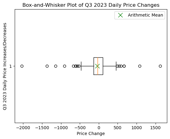
Interpreting the plot:
The box represents the interquartile range (IQR), which covers the middle 50% of the data. The whiskers extend from the box to the minimum and maximum values, excluding outliers.
- The position of the box relative to the whiskers indicates the spread of the price changes and the central tendency of the data.
- The length of the whiskers gives an idea of the range of price changes, excluding outliers.
- Outliers, are visible as individual points outside the whiskers, indicating unusually large price changes.
- The green “x” marks the average daily price change, providing a reference point for the central tendency of the data. Its value is -39.803979230769244
Outlier Detection in Q3 2023 Daily Price Changes
This section determines the number of outliers in the daily price changes during Q3 2023 using vectorized relational operators from NumPy. Outliers are defined based on their deviation from the interquartile range (IQR) according to standard boxplot criteria.
We count the outliers programmatically using vectorized relational operators from NumPy. We need to first define the criteria for identifying outliers. In the context of a boxplot, outliers are defined as data points that fall below the first quartile minus 1.5 times the interquartile range (IQR) or above the third quartile plus 1.5 times the IQR.
# Calculate the first quartile (Q1) and third quartile (Q3)
Q1 = np.percentile(price_changes, 25)
Q3 = np.percentile(price_changes, 75)

# Calculate the interquartile range (IQR)
IQR = Q3 - Q1

# Define the lower and upper bounds for outliers
lower_bound = Q1 - 1.5 * IQR
upper_bound = Q3 + 1.5 * IQR

# Count the outliers
outliers = np.sum((price_changes < lower_bound) | (price_changes > upper_bound))

# Print the result
print("There are", outliers, "outliers.")
There are 16 outliers.Inference
The outliers in the daily price changes could indicate significant deviations from the typical price movements during Q3 2023. These outliers might represent extreme market events, such as sudden price spikes or crashes, anomalies in trading activity, or errors in data recording. Investigating the outliers further could provide insights into unusual market behavior or factors affecting the cryptocurrency exchange rates during that period
Conclusion
Through the analysis conducted in this report, several key insights regarding the BTC-USD exchange rates during Q3 2023 have been obtained:
- The statistical analysis revealed important metrics describing the central tendency, variability, and distribution of exchange rates during the quarter.
- Visualizations provided a graphical representation of the exchange rate trends, aiding in the identification of patterns and anomalies. We leveraged line chart and box and whiskers plot for the same.
- The detection of outliers (16 outliers) in the daily price changes highlighted instances of significant deviations from the typical price movements, suggesting potential market events or anomalies warranting further investigation.
Overall, this analysis offers valuable insights into the dynamics of the BTC-USD exchange rates during Q3 2023, contributing to a better understanding of cryptocurrency market behavior and trends.