The Chosen One - Defining Foundations of Neural Networks

What is a Neural Network

Machine Learning models are functions that fit to a particular data. So, we start with an infinitely flexible function called neural network and then get it to perform a specific task. In this notebook, we will try to define the neural network, specifically gradient descent concept by developing our own mathematical functions.

Let’s start with importing the necessary libraries and creating a user-defined function to plot graph.

# Importing necessary libraries

from ipywidgets import interact
from fastai.basics import *
from functools import partial

# Setting device as mps for Mac M chip series
torch.device('mps')

# Setting dpi (dots per inch) matplotlib plt runtime configuration for figure. 
# [Docs here.](https://matplotlib.org/stable/api/_as_gen/matplotlib.pyplot.rc.html)
plt.rc('figure', dpi=90)

'''
The below function will create a 2 dimensional tensor (x) and plot the function (f) passed as argument.
`torch.linspace(min, max, 100)`: generates a one-dimensional tensor of 100 equally spaced values between min and max.
`[:,None]`: This is a technique used to reshape the tensor. It converts the 1-D tensor into 2-D tensor containing 
            100 rows and 1 column.
You can check the rank of the tensor using len(a.shape)
'''
def plot_function(f, title=None, min=-2.1, max=2.1, color='r', ylim=None, xlim=None):
    x = torch.linspace(min, max, 100)[:, None] # Create rank-2 tensor with 100 elements ranging between `min` and `max
    if ylim: plt.ylim(ylim) # Set the range on y-axis
    if xlim: plt.xlim(xlim) # Set the range on x-axis
    plt.plot(x, f(x), color) 
    if title is not None: plt.title(title)

Fitting a Simple Function to Data

A neural network is just a mathematical function. In the most standard kind of neural network, the function:

Multiplies each input by a number of values. These values are known as parameters
Adds them up for each group of values
Replaces the negative numbers with zeros (ReLU Activation – to be explained later)

This represents one “layer”. Then these three steps are iterated, using the outputs of the previous layer as the inputs to the subsequent layer. Initially, the parameters in this function are selected at random. Therefore a newly created neural network doesn’t do anything useful at all – it’s just random!

To get the function to “learn” to do something useful, we have to change the parameters to make them “better” in some way. We do this using gradient descent. Let’s see how this works…

We will start with fitting a quadratic equation(function) to some datapoints that we will generate randomnly..

The Simple Function … Quadratic

def f(x):
    return 5*x**2 + 4*x + 3

plot_function(f=f, title="Function - $5x^2 + 4x + 3", color='b')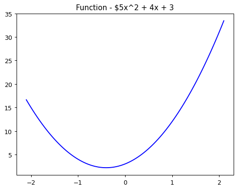

Here 5, 4 and 3 are the parameters or coeffecients for the quadratic function. So, a function \(ax^4 + bx^3 + .. + e\) has a,b,..e as the parameters . All things will get cleared out in sometime. For now, let’s create a python function which takes in parameters and returns value of the function f(x).

def func_quadratic(a, b, c, x):
    return a*x**2 + b*x + c

# Example
func_quadratic(3,4,5,2.5)

33.75

Fix Parameters using Partial

If we fix some particular values of a, b, and c, then we’ll have made a quadratic. To fix values passed to a function in python, we use the partial function. So, what happens is, you fix the values of a,b and c to pass to the function func_quadratic and assign it to a variable say f. We can then call f with whatever values we want to pass to x. Refer below:

def mk_quad(a, b, c):
    return partial(func_quadratic, a, b, c)

f = mk_quad(3,4,5) # Pass values of a,b,c
f(2.5) # Pass value of x

33.75

plot_function(f)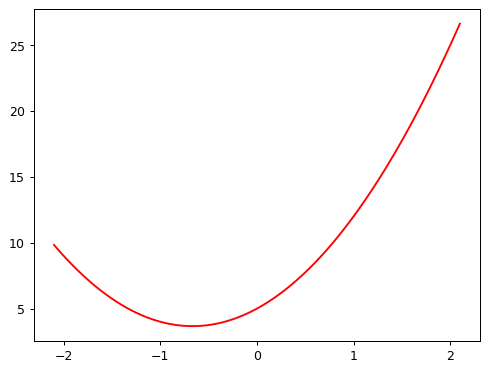

Add Noise to random data

We now try to simulate making some noisy data for our quadratic function f. We can then use gradient descent to see if we can recreate the original function from the data.

from numpy.random import normal, seed, uniform

def noise(x, scale): return normal(scale=scale, size=x.shape)
def add_noise(x, multiplier, add): return x * (1+noise(x,multiplier)) + noise(x,add)

Used normal distributed random numbers to generate noise
Used a custom function to add noise using multiplier and add argument

seed(42)

x = torch.linspace(start=-2, end=2, steps=20)
y = add_noise(f(x), 0.4, 1.5)

x[:5], y[:5]

(tensor([-2.0000, -1.7895, -1.5789, -1.3684, -1.1579]),
 tensor([12.9866,  6.6981,  7.8615,  6.1407,  3.1628], dtype=torch.float64))

As visible, they’re tensors. A tensor is just like an array in numpy. A tensor can be a single number (a scalar or rank-0 tensor), a list of numbers (a vector or rank-1 tensor), a table of numbers (a matrix or rank-2 tensor), a table of tables of numbers (a rank-3 tensor), and so forth.

We’re not going to learn much about our data by just looking at the raw numbers, so let’s draw a picture:

plt.scatter(x,y)
plt.show()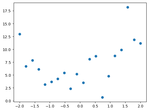

Now, let’s try to use some cool python interactive functions to fit values of a,b and c to fit a line to the datapoints.

Fit the data interactively

@interact(a=1.1, b=1.1, c=1.1)
def plot_quad(a, b, c):
    plt.scatter(x,y)
    plot_function(mk_quad(a,b,c), ylim=(-3,13))

Now we can try on tweaking a, b,& c but this is a tedious task, maybe fun, lol. We defintely would have more than 3 parameters (or coeff) in a real world data and it’s gonna take a lot of time. So, we use Gradient descent to achieve the same. Before creating our gradient descent algorithm, it is notable that one thing that’s making this tricky is that we don’t really have a great sense of whether our fit is really better or worse. It would be easier if we had a numeric measure of that. On easy metric we could use is mean absolute error – which is the distance from each data point to the curve: Solet’s define a loss function, which would be MSE (Mean Squared Error) in this case.

def mae(preds, acts):
    return (torch.abs(preds-acts)).mean()

@interact(a=1.1, b=1.1, c=1.1)
def plot_quad(a, b, c):
    f = mk_quad(a,b,c)
    plt.scatter(x,y)
    loss = mae(f(x), y)
    plot_function(f, ylim=(-3,12), title=f"MAE: {loss:.2f}")

The Gradient Descent Process Automation

We can use calculus to figure out, for each parameter, whether we should increase or decrease it. For this part, we just need derivatives (and not the might wrathy Integration!!). Derivative measures the rate of change of a function. We don’t even need to calculate them ourselves, because the computer will do it for us! An awesome calculus resource: videos by Professor Dave.

The Basic Idea

If we know the gradient of our mae() function with respect to our parameters, a, b, and c, then we know how adjusting (for instance) a will change the value of mae(). If, say, a has a negative gradient, then we know that increasing a will decrease mae(). Then we know that’s what we need to do, since we trying to make mae() as low as possible.

So, we find the gradient of mae() for each of our parameters, and then adjust our parameters a bit in the opposite direction to the sign of the gradient.

To do this, first we need a function that takes all the parameters a, b, and c as a single vector input, and returns the value mae() based on those parameters:

def quad_mae(params):
    f = mk_quad(*params)
    return mae(f(x), y)

quad_mae([1.1, 1.1, 1.1])

tensor(4.6392, dtype=torch.float64)

This is the original MAE without any gradient descent performed.

Doing it from Scratch

Let’s create a randomly initialized parameters with no meaning whatsoever, and store it as a rank-1 tensor.

abc = torch.tensor([1.1,1.2,1.3])
abc

tensor([1.1000, 1.2000, 1.3000])

Our objective is to calculate the gradient, and update the parameters in the direction opposite to the gradient. There’s a very handy way in pytorch to fetch the gradient. We can just simply use requires_grad_() for the tensor to give a heads up! Hey tensor, we will be needing gradient soon :)

abc.requires_grad_()

tensor([1.1000, 1.2000, 1.3000], requires_grad=True)

Let’s now calculate the loss for the provided parameters through our function defined before.

loss = quad_mae(abc)
loss

tensor(4.4666, dtype=torch.float64, grad_fn=<MeanBackward0>)

Hey Pytorch…Now go ahead and do the calculation for me to compute the gradient !

loss.backward()

The above command adds an attribute called grad which gives the gradient.

abc.grad

tensor([-1.4194,  0.0737, -0.9000])

What does the above grad mean ?

It simply means.. (1) if I increase a, loss will go down; (2) if I increase b, loss will go up, (3) if I increase c, loss will go down but very less.

So, now let’s increase a, then increase c and then decrease b.

But how do we do that ? Turns out, the idea is rather simple! If we subtract the gradient, multiplied by a small number, that should improve the outcome and decrease the loss by a bit.

'''
We are updating the parameters by subtracting the gradient times a small number from initial params
'''
with torch.no_grad():
    abc -= abc.grad*0.01
    loss = quad_mae(abc)
    
print(f'loss = {loss:0.3f}')

loss = 4.438

As you can see, the loss has decreased by a very slight amount, i.e., from 4.4666 to 4.438

Also, the interesting code of line with torch.no_grad(): … what is it ?

So, abc.requires_grad_() means, we are instructing pytorch to use the gradient of abc when used in a function ahead. However, in the above code, we don’t really want it’s gradient only. We are updating the parameters here, and hence the above line of code indicates, that don’t use the gradient of abc inside that context manager unless specificallly asked using abc.grad. BAM!!!

The “small number” we multiply is called the learning rate, and is one of the most important hyper-parameter to set when training a neural network.

BTW, you’ll see we had to wrap our calculation of the new parameters in with torch.no_grad(). That disables the calculation of gradients for any operations inside that context manager. We have to do that, because abc -= abc.grad*0.01 isn’t actually part of our quadratic model, so we don’t want derivitives to include that calculation.

We can use a loop to do a few more iterations of this:

for i in range(8):
    loss = quad_mae(abc)
    loss.backward()
    with torch.no_grad(): abc -= abc.grad*0.01
    print(f'step={i}; loss={loss:.2f}')

step=0; loss=4.44
step=1; loss=4.38
step=2; loss=4.30
step=3; loss=4.18
step=4; loss=4.04
step=5; loss=3.87
step=6; loss=3.67
step=7; loss=3.45

abc

tensor([1.7387, 1.1668, 1.7050], requires_grad=True)

If we keep running this loop for looooong time we’ll observe that the loss eventually starts increasing for a while. That’s because once the parameters get close to the correct answer, our parameter updates will jump right over the correct answer! To avoid this, we need to decrease our learning rate as we train. This is done using a learning rate schedule, and can be automated in most deep learning frameworks, such as PyTorch.

But wait.. this doesn’t look powerful enough! Let’s introduce activation Function

Neural network is a very expressive function! It’s poweful and convenient and gets your job done! In fact – it’s infinitely expressive. A neural network can approximate any computable function, given enough parameters. A “computable function” can cover just about anything you can imagine: understand and translate human speech; paint a picture; diagnose a disease from medical imaging; write an essay; etc…

But how does a neural network approximates a function ?

The fundamental steps include (but are not limited to):

Matrix multiplication, which is in layman terms multiplying numbers together and then adding them up
The function \(max(x,0)\), which replaces all negative numbers with zero.

The combination of a linear function and this max() is called a rectified linear function (ReLU), and it can be implemented like this:

def rectified_linear(m,b,x):
    y = m*x+b
    return torch.clip(y, 0.)

The linear function above is \(y=m*x+b\)
In PyTorch, the function \(max(x,0)\) is written as torch.clip(x,0).

f = partial(rectified_linear, 1, 1) # PRoviding *m* and *b*
plot_function(f, title = 'Simple ReLU graph', color = 'g')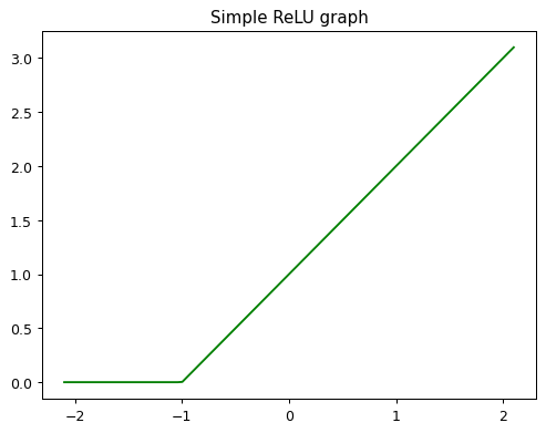

Let’s interact the above function

@interact(m=1, b=2)
def plot_relu(m, b):
    plot_function(partial(rectified_linear, m, b), title='Interactive ReLU', min = -5, color = 'b')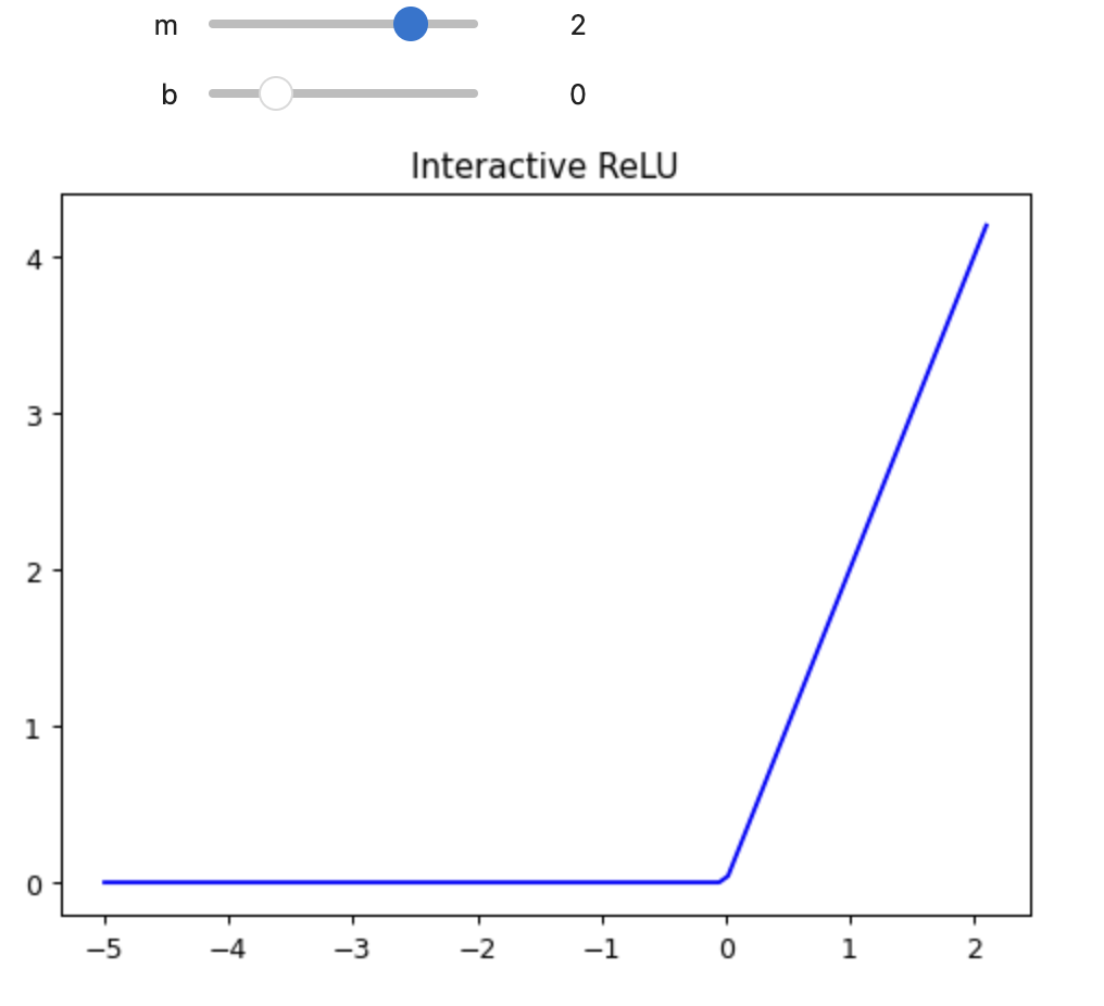

But why is it interesting ?

It’s not!! It isn’t interesting or poweful on it’s own. However, it is awesomly flexibile when we add another layer of ReLU to this graph. Let’s see how..

def double_relu(m1, b1, m2, b2, x):
    return rectified_linear(m1, b1, x) + rectified_linear(m2, b2, x)

@interact(m1=-1.5, b1=-2.0, m2=1.5, b2=1.7)
def plot_double_relu(m1, b1, m2, b2):
    plot_function(partial(double_relu, m1,b1,m2,b2), color = 'b', min = -5, ylim=(-1,6))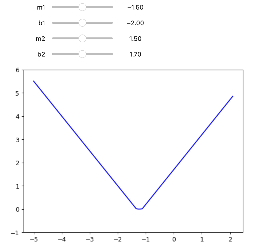

Let’s another layer of ReLU and observe..!

def triple_relu(m1, b1, m2, b2, m3, b3, x):
    return rectified_linear(m1, b1, x) + rectified_linear(m2, b2, x) + rectified_linear(m3, b3, x)

@interact(m1=-1.5, b1=-2.0, m2=1.5, b2=1.7, m3=-1.1, b3=2.0)
def triple_relu(m1, b1, m2, b2, m3, b3):
    plot_function(partial(triple_relu, m1,b1,m2,b2,m3,b3), color = 'b', min = -5, ylim=(-1,10))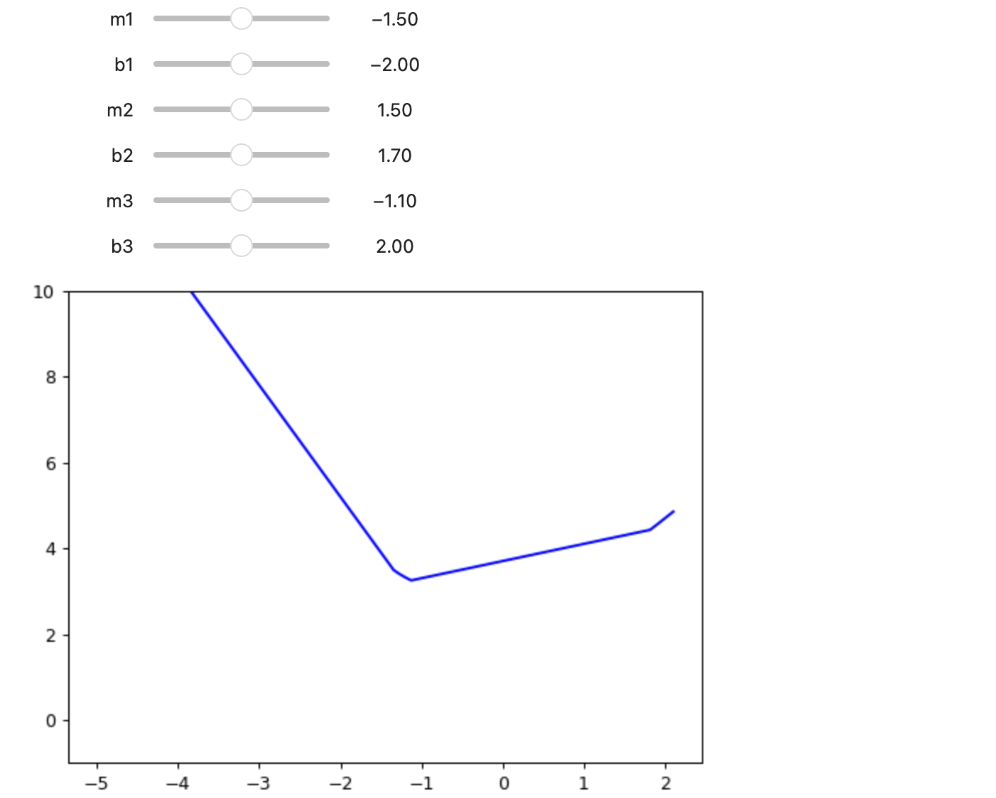

So, we can add as many ReLUs as we want and fit the function as close as we want. Hence, Neural networks are infinitely flexibile functions and can approximate to any input as we like!!

Defining Foundations of Neural Networks - Python